3D Surface Rendering in Postscript
J.
Scott
Drader,
Math
308,
Fall
2003
Contents
- Introduction
- Bezier
Curve Review
- Tensor
Product
Patches
- Bezier
Triangle
Patches
- Other
Representations
- Bibliography
- surface3d.ps
Reference
1.
Introduction
Bezier curves have proven to be a very useful method of modeling
surfaces in many applications. We will assume the reader is familiar
with Bezier curves,
Bernstein
polynomials,
and the DeCasteljau algorithm. We only review the definition and
properties
of Bezier curves, rather
than derive them (section 1). We will focus on two surface representations based on Bezier
curves
(section
2); tensor product surfaces (section
3), and Bezier triangles (section
4).
We will discuss the properties
they
inherit from Bezier curves,
as
well
as
methods for
subdividing
and
rendering them.
Finally
we
mention
some
other
more
complex
representations
not
dealt
with
here
and
why
they
are
desirable
(section
5).
The final section details the provided libraries that were
used to produce
the
images
shown. The libraries provide
methods for Bezier curves in 2D and 3D, as well for tensor product surfaces and
Bezier triangles. The 3d portion the library is built on top of ps3d.inc.
2.
Bezier Curve Review
Definition
Bezier curves can be described on a high-level by their
geometric interpretation, and indeed this is the
property that makes them so elegant. A Bezier curve is a function defined over a single
parameter that interpolates a sequence of points. As the parameter changes, the
path of the line created goes from the first point in the sequence to the last,
moving a long curve that is influenced intuitively by the intermediate control
points.
Recall that Bezier curves use the Bernstein
polynomials as basis functions. The number of
points that are interpolated determine the degree of the curve (and the degree
of the polynomial that interpolates them). The equation of the curve
is
where bi is the ith
control point (i.e. the vector b is the control polygon) and Bim(t)
is the ith Bernstein polynomial of degree m. As
the parameter t varies from 0 to 1, f(t) traverses the curve.
Properties
Bezier curves have several key properties (inherent from the
Bernstein polynomials) that are important to the properties curves and 3D
surfaces based on them. As we are concerned with 3D surfaces we only state the
properties and do not prove them.
-
The curve interpolates its first and last control
point.
-
The entire curve lies within the convex hull of the
control points.
-
It is invariant under affine transformations (i.e. transforming
the curve is only a matter of transforming the control points)
-
The curve is tangent to its control polygon at the
endpoints.
-
The curve can be evaluated and/or subdivided
recursively by the DeCasteljau algorithm.
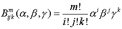
A
degree
3
(cubic)
Bezier
curve
and
its
control
polygon.
Subdivision and Rendering
There are several methods of drawing Bezier curves. The most
obvious method is to directly evaluate the polynomial at fixed intervals of t
to produce a set of points on the curve, which can be joined to form an approximation
of the curve. Although this method works, it is inefficient. The above method
can be sped up by using the recursive DeCasteljau
algorithm to
evaluate the curve for values of
t. The best method however is
recursively subdividing the curve by repeated applications of DeCasteljau.
The DeCasteljau has the property that evaluation of the curve
for a value of
t produces control points for 2 smaller curves, one from 0 to t
and the 2nd from t to 1. Hence applying it at t = 1/2
splits the curve into a left and right curve. By recursively splitting the
original curve, the polygon formed by
assembling
the
control points of
the
sub-curves
quickly converges to the final curve.
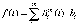
After
2
subdivisions,
the
curve
is
already
closely
approximated
by
the
control
polygons
of
the
4
resultant
curves.
3.
Tensor Product
Patches
Definition
Just as we can use a parameterization in one variable to
define a curve, we can use a parameterization in 2 variables to define a
surface in 3D. Tensor product surfaces (or
rectangular
Bezier
patches) are the 2-variable
extension of Bezier curves. Instead of interpolating a sequence of points, they
can be thought
as
a
way
to
interpolate a sequence of Bezier curves, or a rectangular
mesh of control points. The formula is
where bi,j is the i,jth
control point in the control mesh (i.e. b is the 2D mesh of control
points, which we will refer to as the control net). Holding the parameter s
constant and traversing the surface for 0 <
t < 1 traces a Bezier curve
that lies on the surface, and vice versa.
Properties
The properties of tensor product surfaces are natural extensions of those for
Bezier curves. They are listed below, and numbered such that they correspond to
the above list of properties of Bezier curves.
-
The patch interpolates the corner vertices of its
control net.
-
The surface lies within the convex hull of its control
points.
-
It is invariant under affine transformations (i.e. transforming
the surface is only a matter of transforming the control net).
-
At its corners, the surface is tangent to the vectors
formed by the corner control point and the nearest control points on the
adjacent edges.
-
The patch can be evaluated and/or subdivided
recursively by applying the DeCasteljau algorithm once in each parameter
direction.
-
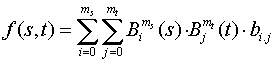
A
rectangular
patch
(degree
2
in
s
and
3
in
t)
and
its
control
polygon.
Subdivision and Rendering
Rendering of tensor product surfaces is also analogous to the
curve case, with the exception that everything has to be done twice, once in
each parameter. We again have direct computation of the polynomial and direct
computation with DeCasteljau's algorithm as options, but subdivision is
attractive again. Just as a Bezier curve can
be split into 2 separate but equivalent curves by a single application of the
DeCasteljau algorithm, a rectangular patch surface can be split into 4 smaller
but equivalent patches (a split in each parameter direction). The parameter
which is chosen first does not affect the result. Rendering via subdivision is
also fairly similar to the Bezier curve case. The obvious difference is that it
is no longer a matter of simply connecting control points, and normal vectors
are required for realistic shading.
There is more than one way to obtain a triangulation of the
surface after having subdivided a patch into several sub-patches. One way is to
render each sub-patch by creating a triangulation of its control mesh, and
computing normals based on the vertices of the each resulting triangle. This
method is fine when only a wireframe approximation of the surface is needed, or
when normals only need to be provided
per-triangle rather than per-vertex.
A
second and arguably more "correct" way is to
render each sub-patch as two triangles (composed of the 4 corner control points
of the subpatch). Note that this scheme does not make use of the interior
control points patches, and hence would typically require an extra subdivision
or two to obtain an equivalently dense triangle mesh. The reason it is often the
favorable method is because exact normal vectors can be obtained at all vertices
used in the triangulation (see property 4 above) which is
ideal
for renderers
requiring per-vertex normals.
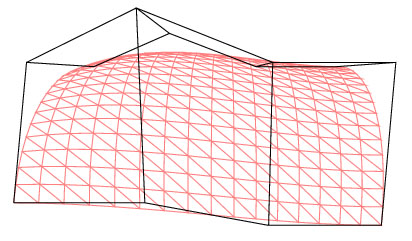
The
triangulation
and
normals
after
2
subdivisions
Refinement
of
a
rectangular
patch
through
subdivision
4.
Bezier
Triangle
Patches
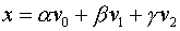
Definition
Bezier triangles are not as simple as tensor product patches.
Rather
than
using
s
and
t
as
parameters
as
in
the
tensor
patch
case,
points
on
the
curve
are
parameterized
with
Barycentric
coordinates.
Given
a
parameter
domain
bounded
by
v1,
v2,
and
v3,
a
point
x
inside
the
domain
can
be
described
as
a
weighting
of
the
vi
:

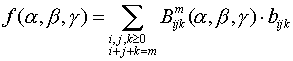
Given
this
parameterization,
the
basis
functions
required
are
the 3-dimensional Bernstein
polynomials,
which
are
defined
as
and
this
gives
us
the
final
equation
for
the
curve:
Properties
The
properties
we
are
interested
in
are
virtually
identical
to
those
listed
above
for
tensor
product
surfaces,
with
the
notable
difference
that
the
DeCasteljau
algorithm
has
a
slightly
different
form
with
the
Barycentric
parameterization.
Subdivision and Rendering
The DeCasteljau algorithm in this case subdivides the control mesh into 3
sub-meshes as follows:
Unlike
with
Bezier curves or tensor product patches however, repeated applications
of this
subdivision
scheme
do not produce a triangulation that approaches the
original
surface
since the edges of the patch are not
refined. A
more
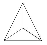
complex algorithm that splits the mesh into the configuration below is possible.
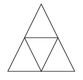
The naive algorithm to do so requires 12 calls to the DeCasteljau algorithm,
but it
can
be
done
in
4
calls
by
using
a
clever
sequence
of
splits.
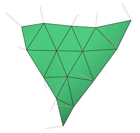
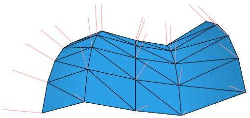
The
triangulation
and
normals
of
a
cubic
Bezier
triangle
after
2
subdivisions
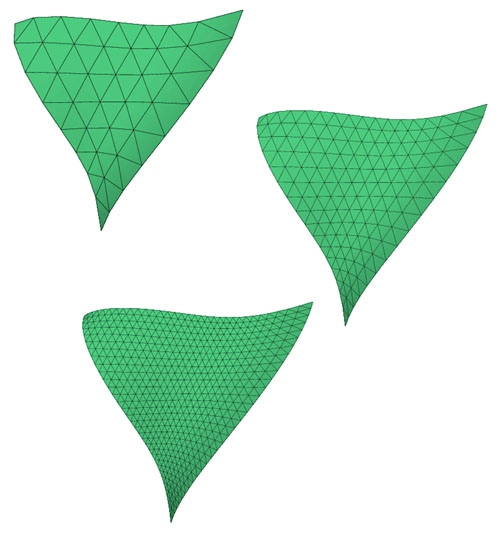
Refinement
of
a
triangular
patch
through
subdivision
5.
Other Representations
An
often
desirable
but
difficult
to
deal
with
task
that
we
have
not
discussed
involves
joining
curves
or
patches
into
more
complex
curves
or
patches.
Typical
reasons
for
combining
several
curves
or
patches
include
the
desire
to
assemble
more
complex
surfaces,
and
the
desire
to
achieve
more
locality
of
control
(i.e.
a
control
point
affects
only
the
part
of
the
curve
closest
to
it).
The
fundamental
problem
that
arises
in
attempting
to
to
achieve
either
of
these
ideals
is
linking
the
curves
or
patches
in
a
continuous
fashion.
Constraints
placed
on
neighboring
curves
or
patches
of
the
type
we
have
discussed
can
be
fairly
easily
derived
for
each
of
the
the
representations
via
their
polar
forms,
but
this
is
beyond
our
scope,
and
provides
a
good
starting
point
for
further
reading.
Representations
that
we
have
not
mentioned
that
begin
to
deal
with
these
problems
by
implicitly
enforcing
the
continuity
constraints
include
B-Splines,
rational
curves,
NUBS
(Non-Uniform
B-Splines)
and
NURBS
(Non-Uniform
Rational
B-Splines).
6.
Bibliography
Gallier,
J.,
Curves
and
Surfaces
in
Geometric
Modelling,
Morgan
Kaufmann
Publishers,
Sanfrancisco,
CA,
2000.
Heidrich,
W.,
Geometric
Modelling,
http://www.ugrad.cs.ubc.ca/~cs424/Slides/index.shtml
Akenine-Möller,
T,
Haines,
E,
Bezier Triangles and N-Patches,
http://www.gamasutra.com/features/20020715/mollerhaines_01.htm
Kruger,
G,
Curved
Surfaces
Using
Bezier
Patches,
http://www.gamasutra.com/features/19990611/bezier_01.htm
7.
surface3d.ps
Reference
surface3d.inc
is
a
library
for
rendering
Bezier
curves,
tensor
product
patches,
and
Bezier
triangles
in
PostScript.
Methods
are
provided
for
evaluation,
subdivision,
and
rendering.
surface3d.inc
makes
use
of
ps3d.inc
and
it
is
assumed
they
are
in
the
same
directory.
Structures
There
are
4
main
structures
used
by
surface3d.inc.
They
are
detailed
below:
| Structure
Name: |
bez3 |
| Description: |
The
control
polygon
for
a
3d
Bezier
curve |
| Structure: |
[
b1
...
bn
];
where
the
degree
of
the
curve
is
n
-1 |
| Structure
Name: |
rpatch |
| Description: |
The
control
polygon
for
a
tensor
product
surface |
| Structure: |
[[b1,1
...
b1,m]
...
[bn,1
...
bn,m]];
where
the
patch
is
degree
n
-1
in
s
and
m
-
1
in
t |
| Structure
Name: |
tpatch |
| Description: |
The
control
polygon
for
a
Bezier
triangle |
| Structure: |
[[b1,1]
...
[bn,1
...
bn,n]];
where
the
patch
is
degree
n
-1 |
| Structure
Name: |
frag |
| Description: |
A
triangular
surface
fragment. |
| Structure: |
[[v1
n1]
[v2
n2]
[v3
n3]];
where
vi
are
the
vertices
and
ni
their
normal
vectors |
Methods
bez3
methods:
| Method
Name: |
bez3-eval |
| Description: |
Evaluates
a
Bezier
curve
at
a
given
value
of
t |
| Parameter(s): |
bez3
t;
the
Bezier
and
the
parameter
value |
| Return
Value(s): |
v;
the
point |
| Method
Name: |
bez3-subdiv |
| Description: |
Subdivides
a
Bezier
curve
at
a
given
value
of
t. |
| Parameter(s): |
bez3
t;
the
Bezier
and
the
parameter
value |
| Return
Value(s): |
bez-left
bez-right;
the
2
resultant
Beziers |
| Method
Name: |
bez3-subdiv-arr |
| Description: |
Recursively
subdivides
an
array
of
Beziers
at
t
=
0.5 |
| Parameter(s): |
bez3-arr
n;
the
array
of
Beziers
and
the
number
of
subdivisions
to
perform |
| Return
Value(s): |
bez3-arr-new;
the
new
array
of
Beziers |
| Method
Name: |
bez3-build-path-arr |
| Description: |
Builds
a
path
for
an
array
of
Beziers |
| Parameter(s): |
bez3-arr;
the
array
of
Beziers |
| Return
Value(s): |
none |
rpatch
methods:
| Method
Name: |
rpatch-eval |
| Description: |
Evaluates
a
rectangular
patch
for
given
values
of
s
and
t. |
| Parameter(s): |
rpatch
s
t;
the
Bezier
and
the
parameter
values |
| Return
Value(s): |
v;
the
point |
| Method
Name: |
rpatch-subdiv |
| Description: |
Subdivides
a
rectangular
patch
into
4
patches |
| Parameter(s): |
rpatch;
the
patch |
| Return
Value(s): |
rpatch1
rpatch2
rpatch3
rpatch4;
the
4
resultant
patches |
| Method
Name: |
rpatch-subdiv-arr |
| Description: |
Recursively
subdivides
an
array
of
rectangular
patches
(into
4
patches
each) |
| Parameter(s): |
rpatch-arr
n;
the
array
of
patches
and
the
number
of
subdivisions
to
perform |
| Return
Value(s): |
rpatch-arr-new;
the
new
array
of
patches
after
n
subdivisions |
| Method
Name: |
rpatch-build-path-arr |
| Description: |
Built
a
path
representing
the
control
meshes
of
an
array
of
patches |
| Parameter(s): |
rpatch-arr;
the
array
of
patches |
| Return
Value(s): |
none |
| Method
Name: |
rpatch-get-fragments-arr |
| Description: |
Returns
an
array
of
fragments
representing
the
array
of
patches |
| Parameter(s): |
rpatch-arr;
the
array
of
patches |
| Return
Value(s): |
frag-arr;
the
array
of
fragments |
tpatch
methods:
| Method
Name: |
tpatch-rotate |
| Description: |
Rotates
a
patch
rst
to
str |
| Parameter(s): |
rst;
the
patch |
| Return
Value(s): |
str;
the
rotated
patch |
| Method
Name: |
tpatch-transpose |
| Description: |
Takes
the
patch
rst
and
computes
its
transpose,
rts |
| Parameter(s): |
rst;
the
patch |
| Return
Value(s): |
rts;
the
transposed
patch |
| Method
Name: |
tpatch-eval |
| Description: |
Evaluates
a
patch
for
given
Barycentric
coordinates |
| Parameter(s): |
tpatch
[alpha
beta
gamma];
the
patch
and
Barycentric
coordinates |
| Return
Value(s): |
v;
the
point |
| Method
Name: |
tpatch-subdiv-3 |
| Description: |
Subdivides
a
triangular
patch
into
3
patches
for
the
given
Barycentric
coordinate |
| Parameter(s): |
rst
[alpha
beta
gamma];
the
patch
and
Barycentric
coordinates |
| Return
Value(s): |
ars
ast
atr;
the
3
resultant
patches |
| Method
Name: |
tpatch-subdiv-4 |
| Description: |
Subdivides
a
patch
into
4
patches
for
Barycentric
coordinates
[1/3
1/3
1/3] |
| Parameter(s): |
rst;
the
patch
to
be
subdivided |
| Return
Value(s): |
bas
cra
cab
cbt;
the
4
resultant
patches |
| Method
Name: |
tpatch-subdiv-arr |
| Description: |
Recursively
subdivides
an
array
of
patches
(into
4
patches
each) |
| Parameter(s): |
tpatch-arr
n;
the
array
of
patches
and
the
number
of
subdivisions
to
be
performed |
| Return
Value(s): |
tpatch-arr-new;
the
new
array
of
patches
after
n
subdivisions |
| Method
Name: |
tpatch-get-fragments-arr |
| Description: |
Returns
an
array
of
fragments
representing
the
array
of
patches |
| Parameter(s): |
tpatch-arr;
the
array
of
patches |
| Return
Value(s): |
frag-arr;
the
array
of
fragments |
frag
methods:
| Method
Name: |
draw-fragments-gouraud |
| Description: |
Draws
an
array
of
fragments
with
Gouraud
shading |
| Parameter(s): |
frag-arr
light-source
shade-func
color;
the
array
of
fragments,
a
4-value
array
reprsenting
the
light
source,
a
4-value
array
representing
the
shading
curve,
a
3-value
array
representing
an
RGB
color |
| Return
Value(s): |
none |
| Method
Name: |
build-fragments-wireframe |
| Description: |
Built
a
path
representing
the
edges
of
an
array
of
fragments |
| Parameter(s): |
frag-arr;
the
array
of
fragments |
| Return
Value(s): |
none |
| Method
Name: |
build-fragment-normals |
| Description: |
Built
a
path
representing
the
normal
vectors
of
an
array
of
fragments |
| Parameter(s): |
frag-arr
len;
the
array
of
fragments,
the
length
the
normals
are
to
be
drawn |
| Return
Value(s): |
none |