Mathematics 309 - Adaptive Optics and the Use of Mirrors

This webpage is meant to convey the mathematics behind the use of deformable mirrors in adaptive optic systems and not as a comprehensive explanation of adaptive optic systems themselves. References used are mentioned at the bottom and they seem to be very friendly introductions for those with limited physics backgrounds like myself.

Topics covered:

Part I- A Brief Overview of How Adaptive Optic Systems Work
Part II - A Review of Phase Shifting/Conjugation and Basic Mirror Reflection
Part III - A look at Deformable Mirrors in More Detail
Part IV - References

Part I - A Brief Overview of Adaptive Optic Systems

Adaptive optic (AO) systems developed for imaging systems help provide a clearer image from the data gathered from these systems by essentially shifting the phase of optic waves coming in.

AO systems can be characterized by three main components: a deformable mirror, a wavefront sensor, and a control computer. These components work together to measure the distortion caused by the environment and to adjust incoming data to minimize the effects of these distortions. In principle, the wavefront sensor collects data about the phase of the wavefronts and sends this data to the control computer which translates these signals and sends these commands to change the shape of the mirror so that when the data hits the mirror, its phase is altered almost as if the environment had never interfered with its signals.

A simplistic view of the general adaptive optic system is shown below:

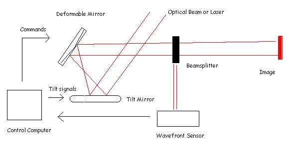
Figure 1: Adaptive Optics Simplified System (created in MS Paint)

Systems vary and can incorporate numerous other gadgets such as the telescope. AO has helped astronomers map the sky a little more...and has enabled the largest ground telescopes in the world to obtain images exceeding the quality of those obtained from the Hubble Telescope in the sky. Back to top

A Review of Phase Shifting/Conjugation and Basic Mirror Reflection

The idea of phase shifting and conjugation (we are adding the conjugate of A exp(-i*phi) to the optical beam's electric field) can be simply explained by looking at graphs of waves.

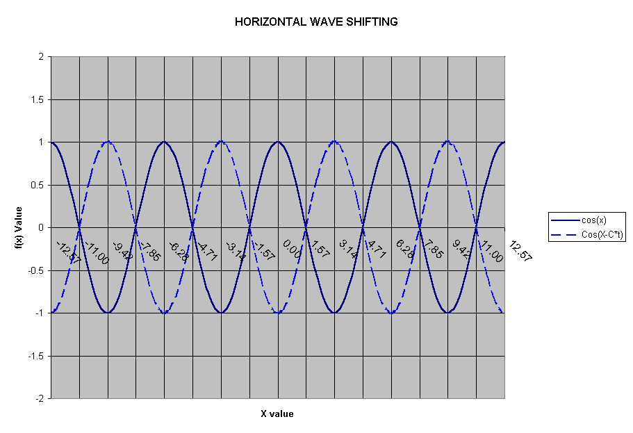
Figure 2: Example of waves out of phase (from Assignment #1)

The equations of the wave f(x) and f(x-ct) are shown.
We see that these two waves are out of phase by 1.58 units in the x-direction and can be made back in phase by shifting one of the waves by 1.58 units.

That's it in a nutshell!

Before we get onto deformable mirrors, here's a review of the basic rules with respect to how light reflects off of mirrors.

In the figure below, there is one flat, one convex, and one concave mirror shown left to right.

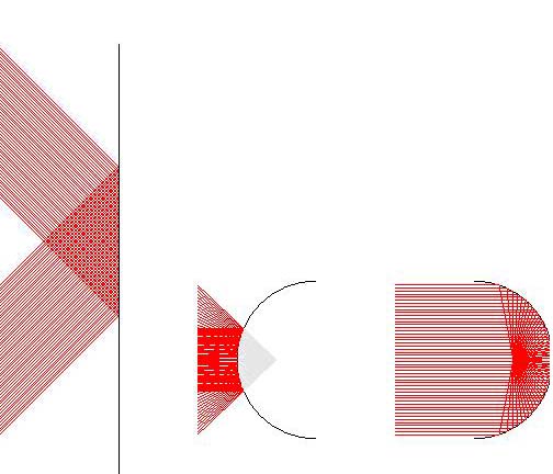
Figure 3: The rules of mirror reflection: flat (l), convex (middle), concave (r) mirrors (created in Matlab)

Rules for Flat Mirror:

Rules for Convex Mirror:

Rules for Concave Mirror:

The above figure applied these rules. Back to top

Part III - A look at Deformable Mirrors in More Detail

The logic behind deformable mirrors is very simple, and yet the mathematics is complicated. We try now to explain what goes on when an optical beam hits the mirror.

Let us think about light as rays, for a second. This wave phase-shifting can almost be seen as an analogy to the following scenario: suppose we have a lens that has a focal plane f.

Figure 4: One lens (created in PostScript)

We put another lens in the path between the original lens and its focal plane.

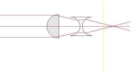
Figure 5: Another lens in the path of the rays, causing focal point to move - undesirable (created in PostScript)

We now have rays being focussed onto a different point. We want to be able to refocus these rays back to their original focal point without taking anything away from the lens system. That would be placing another lens somewhere so as to compensate for this aberration. This is essentially what deformable mirrors do in the adaptive optics system. Along with the other major components of the adaptive optic systems, they take images distorted by the environment and make them more distinct.

An illustration of this idea:

Before: After:
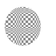
Figure 6 & 7: A Blurry and non-blurry image (created in Photoshop)

So, we deal with light as waves instead of rays, and play around with the electromagnetic properties of light. The electric field of these waves is represented by the equation:

A exp(-i * phi )

where A represents the amplitude of the wave, i is the square root of -1 (yes, we use a complex number), and phi is the phase shift.

When the light waves come in from the environment, atmospheric distortion causes them to arrive somewhat out of phase. In order to put these waves back in phase, we must correct the field by adding the equivalent of a shift by the conjugate of A exp(-i * phi )...that is, A exp(i * phi).

Many types of mirrors have been developed - segmented mirrors, bimorph (voltage is applied) mirrors, and of course - continous surface deformable mirrors.

These continous surface mirrors have electronmechanical actuators (changes the shape of the mirror) behind them that deform the surface of the mirrors. The actuators each affect the surface of the mirror within a radial distance that can be approximated by the equation:

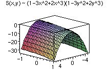
Figure 8: A cubic estimate of the influence function of actuators (Drawn using Maple)

which is also called an Influence function. This can also be characterized by other different equations, depending on what affects the actuator and its influence on the surrounding mirror surface.

To best explain how deformable mirrors work, we look at an example (taken from Introduction to Adaptive Optics).

We are given wavefront signals from the wavefront sensor and must calculate the commands to send to the actuators in the mirror.

The control computer computes signals that will be used to deform the mirror. This is in the form of simple commands to each actuator to move (or not), by how much and in which direction. For our purposes, we will start with the slope calculations carried out by the control computer. This boils down to the simple equation:

y = Ax

where y represents the slopes calculated from the wavefront signals, x represents the commands to the actuator, and A is a matrix that takes into account the influence function of the actuators. A is an NxM matrix, where N = number of actuators and M = number of wavefront signals.

Suppose 3 actuators are positioned at (xn, yn) of a mirror. Using the influence function,

exp( -1.9/ 2 * ((x - xn)^2 + (y-yx)^2) )

we come up with the integral:

S(x, a) = integral(x * I(x, y) dx

where I(x, y) is the influence function just mentioned above.

We evaluate this integral S(x, a) over the lowest and highest positions of the actuators to get the following linear system s=Ba:

[s1x] = [0.45  0.088  -0.45] [a1 a2 a3]'
[s2x] = [0.088 0.45   -0.45]
[s1y] = [0.45  -0.26  -0.45]
[s2y] = [0.26  0.45    0.45]
[p]   = [1     1       1   ]

a = [B'B]^-1 * B' y

we get:

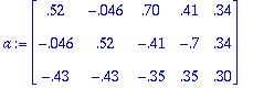
Figure 9 - Matrix that, applied to the measured slopes [s1x s2x s1y s2y p] gives us the commands for [a1 a2 a3].

Let us use this equation. Say p = 0, and our slopes are [1, 1, 1, -1]. Multiplying by the matrix above, we get: . This tells us that actuator 1 and 2 will rise up, while actuator 3 goes down.

That's pretty much it.

Back to top

Part IV - References

Lukin, Vladimir P. Atmospheric Adaptive Optics, SPIE Press, Bellingham (1995).
Tyson, Robert K. Introduction to Adaptive Optics, SPIE Press, Bellingham (2000).
Tyson, Robert K. Principles of Adaptive Optics, Academic Press, Toronto (1991).

....and to a lesser extent:
http://www.cfht.hawaii.edu/Instruments/Imaging/AOB/local_tutorial.html

A good site for reviewing basics of mirror reflection and other physics stuff:
http://www.glenbrook.k12.il.us/gbssci/phys/Class/refln/u13l3a.html

Back to top