Using EXCEL Spreadsheets to Solve a 1D Wave Equation

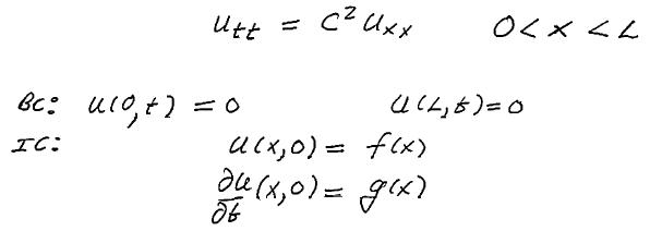
The goal of this tutorial is to describe how to use an EXCEL spreadsheet to compute numerically the solution to the following initial-boundary value problem for the one-dimensional wave equation:

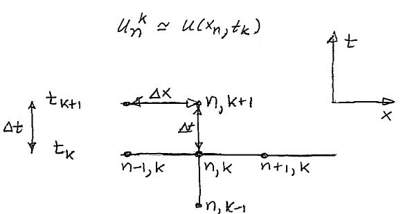
Let us introduce a finite difference mesh x_n = nΔx and t_k = kΔt, and let the corresponding nodal values be denoted by

Derivatives will be approximated by central differences both in space and time,

By rearranging terms, one obtains

where r= (c Δt/Δx).

The resulting discrete equation involves three distinct time levels: known data from steps k - 1 and k are transferred to step k + 1. In other words, to compute the time evolution of the solution its values at both time t_k and an earlier time t_k-1 must be known.

This three-level scheme poses some challenges when imposing the initial condition. To calculate the value of u_n at the first time step k = 1, one needs information from step k = - 1 and k = 0. The initial condition u(x, 0) = f(x) provides information at step k = 0. Any information at an earlier time must be inferred. The initial velocity condition can be used to do that. Imagine a row of false mesh point at time t = - Δt = t_-1, then the initial velocity condition can be approximated using central differences as

thus

Assuming that the discrete wave equation also holds at t = 0, one can compute the value of the solution at time t = t₁ as

and substitute in the expression for u_n^-1 derived from the initial velocity condition. After re-arranging one obtains

Since u_n⁰=f(x_n) and g(x_n) are known at all nodes, we are now in a position to specify the first two rows of nodes. Let's see how to build an EXCEL spreadsheet that implements this calculation.

In line with the spreadsheet format used in other tutorials, we will be working with a spreadsheet where rows represent time levels, and columns correspond to spatial nodes. In particular, throughout this tutorial we will refer to this spreadsheet.

1. How to Tabulate the Spatial/Time Interval
2. How to Include the Initial Condition
3. How to Compute the First Time Step
4. How to Compute the Solution at Subsequent Time Steps
5. How to Create an Animation of the Solution

Step 1: How to Tabulate the Spatial/Time Interval

Sample points in the spatial interval will be tabulated along row 2, from cell D2 through cell AR2; subsequent time values will be shown in column A.

For this tutorial, consider a spatial interval [0, 1.57], and an increment Δx = 0.04. Note that the value of Δx is stored in cells C1.

As usual, each sample point is calculated as

for n = 1, ... N and x₀ = 0.

Each time level is calculated as

for k = 1, ... M and t₀ = 0, using a time step Δt = 0.01. Note that the value of Δt is stored in cell E1.

Step 2: How to Include the Initial Condition

The next step is to assign the initial condition u(x,0) = f(x). Note that the specific form of f(x) depends on the characteristic of the problem under consideration. For this tutorial, we chose

f(x) = exp(-40(x - π /4)²)

The values of f(x_n) are entered in row 5.

The values of g(x_n) from the initial velocity condition are entered in row 4. For this tutorial, we chose g(x) = 0. These values will be used in computing the first time step, as shown in Step 3.

Step 3: How to Compute the First Time Step

The first time step is computed and stored in row 7. In each cell of row 7 that represents a node, an EXCEL formula is coded to compute the expression

which is obtained by re-arranging the terms in the expression for u_n¹ derived in the introduction of this tutorial. Note that the value of r² is stored in cell I1.

For example, u₁¹ is computed as

and its value is stored in cell E7. The EXCEL formula coded in cell E7 must call the following cells:

• cell E6 to read the value of u₁⁰
• cell E1 to read the value of the time step Δt
• cell E5 to read the value of g(x₁)
• cell I1 to read the value of r²
• cell F6 to read the value of u₂⁰
• cell D6 to read the value of u₀⁰

The resulting formula is E6+$E$1*E5+0.5*$I$1*(D6-2*E6+F6). Note that Δt and r² are constants, thus the cells containing their values are called by absolute referencing using the dollar signs in their cell address.

To compute the solution at the adjacent node, u₂¹, it is sufficient to copy and paste the formula used in cell E7 into the cell to the immediate right, that is, cell F7. Copying and pasting the same formula along row 7 allows you to compute the solution at each node at time t = t₁. Note that the value of the solution on the last node is given by the boundary condition of the problem.

Step 4: How to Compute the Subsequent Time Steps

To compute the solution at later times the recursion formula is implemented

This expression is obtained by re-arranging the terms in the equation for u_n^k+1 derived in the introduction of this tutorial.

For example, u₁² is computed as

and its value is stored in cell E8. The EXCEL formula coded in cell E8 must call the following cells:

• cell E7 to read the value of u₁¹
• cell E6 to read the value of u₁⁰
• cell I1 to read the value of r²
• cell F7 to read the value of u₂¹
• cell D7 to read the value of u₀¹

The resulting formula is 2*E7-E6+$I$1*(D7-2*E7+F7). Again, since r² is a constant, the cell containing its value is called by absolute referencing using the dollar signs in its cell address.

To compute the solution at the adjacent node, u₂², simply copy and paste the formula used in cell E8 into the cell to the immediate right, that is, cell F8. Then, repeat the same procedure to fill in the cells in row 8 to compute the solution at each node at time t = t₂, and similarly, into each row below it to find the time evolution of the initial wave.

The Edit|Fill|Fill Right and Edit|Fill|Fill Down features will allow you to fill in all necessary cells and calculate the solution quickly.

Step 5: How to Create an Animation of the Solution

The wave propagation can be easily observed if one plots the solution computed in the spreadsheet at different time levels. Instead of creating several overlapping graph of u at different t, in EXCEL it is possible to generate an animation that runs through the values of the solution previously calculated in the spreadsheet. This animation is implemented in the spreadsheet described in this tutorial.

First of all, observe the plot shown in Fig 1. It depicts the solution u computed in the spreadsheet over the entire spacial domain at a certain time interval.

A slider has been added in cell X1. By clicking the bar on the slider in cell X1, the plot in Fig 1 changes. As the bar on the slider is moved from left to right, the plots show the time evolution of the wave signal.

Let's see how the animation works. The graph in Fig 1 plots the values stored in row 3, from cell D3 through AR3. To see how these values were generated, consider the formula coded in the cells along row 3. The formulas make use of the function OFFSET( ).

In its simplest version, the function OFFSET returns a reference to a cell that is offset by a certain number of rows and columns from a given cell. Specifically, OFFSET(reference, rows, cols) returns a reference as follows: reference is the cell address from which you want to base the offset; rows is the number of rows, up or down, to be added or removed to or from the cell address of reference; cols is the number of columns, to the left or right, to be added or removed to or from the cell address of reference. For example, if OFFSET(C2,1,2) is coded in a given cell, the value shown in that cell is the value stored in a cell one row below and two column to the right of cell C2, i.e., cell E3.

In the spreadsheet described in this tutorial, the OFFSET function is used in the following manner. The value shown, for example, in cell D3 is generated by OFFSET(D8,$M$1,0), that is, by offsetting the reference D8 by a number of rows equal to the value shown in cell M1, without changing column. When the bar on the slider is all the way to the left, the value in cell M1 is 0. Thus, the OFFSET function coded in cell D3 returns the value in cell D8 offset by 0 rows and 0 columns. In other words, it returns the value in D8, which is u₀². Similarly, the value shown in cell E3 is simply the value read from cell E8, which is u₁², and so forth. So, when the value in cell M1 is 0 the plot in Fig1 shows the solution computed at time t = t₂.

Now observe what happens to cell M1 when the bar on the slider is moved slightly to the left. The value in cell M1 increases to 1, causing the values in row 3 to change. Now the cells in row 3 return the values stored in a row that is offset from row 8 by 1, i.e., row 9. In other words, now row 3 shows the solution computed at time t = t₃. By moving the slider progressively to the left, the cells in row 3 point to subsequent rows and the solution computed at subsequent time steps is plotted in sequence in Fig 1.