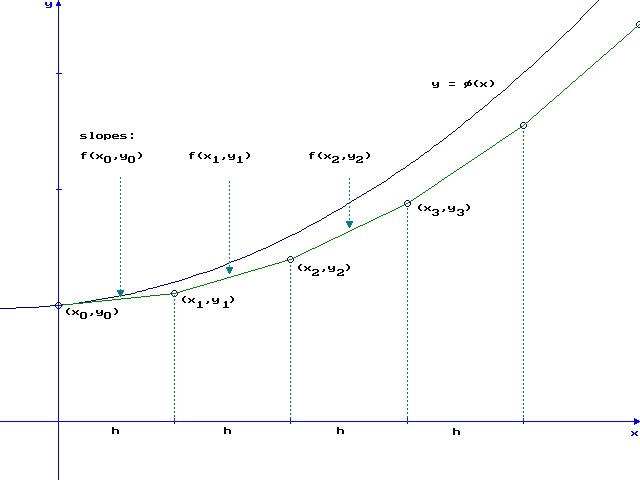
Let's look at an example. We'll consider the initial value problem
![]() ,
, ![]() . This equation is separable, and
the solution turns out to be
. This equation is separable, and
the solution turns out to be
![]() , so we'll be able to
compare the Euler approximation to the true solution.
With step size
, so we'll be able to
compare the Euler approximation to the true solution.
With step size ![]() , we have the following results:
, we have the following results:
![]() ,
,
![]() , etc. By comparison, the true solution has
, etc. By comparison, the true solution has
![]() ,
,
![]() ,
etc. Here is a table of the results of the first 10 steps, which takes
us up to
,
etc. Here is a table of the results of the first 10 steps, which takes
us up to ![]() . (I'm showing 9 digits of the results, but they are
actually being computed in double precision, so roundoff error won't
be a concern)
. (I'm showing 9 digits of the results, but they are
actually being computed in double precision, so roundoff error won't
be a concern)
| Error | |||
| 0.0 | 1.00000000 | 1.00000000 | 0.0 |
| 0.1 | 1.10000000 | 1.10526316 | 0.00526316 |
| 0.2 | 1.21022444 | 1.22222222 | 0.01199778 |
| 0.3 | 1.33223648 | 1.35294118 | 0.02070470 |
| 0.4 | 1.46792616 | 1.50000000 | 0.03207384 |
| 0.5 | 1.61959959 | 1.66666667 | 0.04706708 |
| 0.6 | 1.79009854 | 1.85714286 | 0.06704432 |
| 0.7 | 1.98296335 | 2.07692308 | 0.09395973 |
| 0.8 | 2.20265794 | 2.33333333 | 0.13067539 |
| 0.9 | 2.45488648 | 2.63636364 | 0.18147716 |
| 1.0 | 2.74704729 | 3.00000000 | 0.25295271 |
In an effort to improve our accuracy, we might try a smaller step size.
With ![]() , we get
, we get
![]() . Note that now
. Note that now
![]() , so we should compare this to
, so we should compare this to
![]() .
Then
.
Then
![]() is the approximate
value at
is the approximate
value at ![]() . The next table shows the values
computed with
. The next table shows the values
computed with ![]() for the same
for the same ![]() values as before (thus leaving
out the odd
values as before (thus leaving
out the odd ![]() 's).
's).
| 0.0 | 1.00000000 | 1.00000000 | 0.0 |
| 0.1 | 1.10252967 | 1.10526316 | 0.00273349 |
| 0.2 | 1.21596496 | 1.22222222 | 0.00625726 |
| 0.3 | 1.34209198 | 1.35294118 | 0.01084920 |
| 0.4 | 1.48310373 | 1.50000000 | 0.01689627 |
| 0.5 | 1.64172213 | 1.66666667 | 0.02494454 |
| 0.6 | 1.82136643 | 1.85714286 | 0.03577643 |
| 0.7 | 2.02638978 | 2.07692308 | 0.05053330 |
| 0.8 | 2.26241822 | 2.33333333 | 0.07091511 |
| 0.9 | 2.53684738 | 2.63636364 | 0.09951625 |
| 1.0 | 2.85958887 | 3.00000000 | 0.14041113 |
If we compare the errors with ![]() to the errors at the same points
with
to the errors at the same points
with ![]() , we see that we have approximately halved each of these
errors (the actual ratio ranges from about
, we see that we have approximately halved each of these
errors (the actual ratio ranges from about ![]() to
to ![]() ).
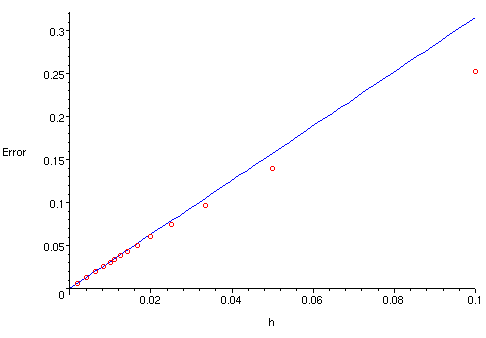
In the graph below we show the error in the Euler approximation at
).
In the graph below we show the error in the Euler approximation at
![]() as a function of the step size
as a function of the step size ![]() .
We use 14 different values for
.
We use 14 different values for ![]() :
: ![]() ,
, ![]() ,
, ![]() ,
, ![]() ,
,
![]() ,
, ![]() ,
, ![]() ,
, ![]() ,
, ![]() ,
, ![]() ,
, ![]() ,
, ![]() ,
,
![]() ,
, ![]() (note that we need
(note that we need ![]() to be an integer
to be an integer ![]() so that
so that
![]() will be 1). The data points are shown by circles. Especially for
small
will be 1). The data points are shown by circles. Especially for
small ![]() , they are very close to a straight line through the origin,
representing a constant times
, they are very close to a straight line through the origin,
representing a constant times ![]() .
.

We could try other examples, and the net result would be similar:
the error in the Euler approximation for a given ![]() is approximately proportional to
is approximately proportional to ![]() . We'll see why later.
But the consequence of this is that the Euler method is not suitable
if you want reasonable accuracy. Suppose, in our example, we wanted the
error at
. We'll see why later.
But the consequence of this is that the Euler method is not suitable
if you want reasonable accuracy. Suppose, in our example, we wanted the
error at ![]() to be less than
to be less than ![]() . Approximately what stepsize, and
how many steps, would be
needed?
We had an error of
. Approximately what stepsize, and
how many steps, would be
needed?
We had an error of ![]() with step size
with step size ![]() , and the error is
approximately proportional to the step size. To divide the error by
, and the error is
approximately proportional to the step size. To divide the error by
![]() we would have to divide the step size by the same amount,
so the step size would have to be about
we would have to divide the step size by the same amount,
so the step size would have to be about
![]() .
The number of steps would be about
.
The number of steps would be about
![]() (more than 28 billion).
This would take a significant amount of time, even on a fast computer.
Moreover, there would be severe problems with roundoff error, because
each step would only add a number on the order of
(more than 28 billion).
This would take a significant amount of time, even on a fast computer.
Moreover, there would be severe problems with roundoff error, because
each step would only add a number on the order of ![]() to
to ![]() .
This means about 10 digits of accuracy is lost. Even in double precision,
not enough digits will remain to attain the desired accuracy.
.
This means about 10 digits of accuracy is lost. Even in double precision,
not enough digits will remain to attain the desired accuracy.