Error Analysis of the Euler Method
As before, we are considering the first-order initial value problem
and approximating its solution using Euler's method with a certain
step size  . I will ignore roundoff error and consider only the
discretization error.
For
step-by-step methods such as Euler's for solving ODE's, we want to
distinguish between two types of discretization
error: the global error and the local error.
The global error at a certain value of
. I will ignore roundoff error and consider only the
discretization error.
For
step-by-step methods such as Euler's for solving ODE's, we want to
distinguish between two types of discretization
error: the global error and the local error.
The global error at a certain value of  (assumed to be
 )
is just what we would ordinarily call the error: the difference between
the true value
)
is just what we would ordinarily call the error: the difference between
the true value  and the approximation
  .
The local error at
.
The local error at  is, roughly speaking, the error introduced in
the
is, roughly speaking, the error introduced in
the  th step of the process. That is, it is the difference between
and
th step of the process. That is, it is the difference between
and
 , where
  is the solution
of the differential equation with
is the solution
of the differential equation with
 . Thus if
 were exactly correct (equal to
  ), the global
error at would be equal to this local error. But since in
general is not correct (as a result of earlier local errors),
the global and local errors are different.
In the picture below,
), the global
error at would be equal to this local error. But since in
general is not correct (as a result of earlier local errors),
the global and local errors are different.
In the picture below,  is the black curve,
and the curves
is the black curve,
and the curves  are in red.
The local errors at each stage of the process
are the blue vertical lines.
are in red.
The local errors at each stage of the process
are the blue vertical lines.
First we consider the local error at :
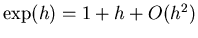
Now
 . According to Taylor's Theorem, for any
twice-differentiable function
. According to Taylor's Theorem, for any
twice-differentiable function 
for some  between and
  . Taking
 ,
,  and
and  we find
If there is some constant  such that we can be sure that
 , then we can say
Such a does exist (assuming  has continuous derivatives in some
rectangle containing the true and approximate solutions):
for any solution of the differential equation
has continuous derivatives in some
rectangle containing the true and approximate solutions):
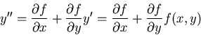
for any solution of the differential equation  , we can differentiate
once more to get
, we can differentiate
once more to get
which is a continuous function of and  and therefore
can't get too big in our rectangle.
and therefore
can't get too big in our rectangle.
Now, what about the global error? It's tempting to say that the
global error at  is the sum of all the local errors
  for
for
 from 1 to . Since each
  and there are
 of them, the global error should be
 .
Unfortunately, it's not quite true that the global error is the sum of the
local errors: the global error at is the sum of the differences
.
Unfortunately, it's not quite true that the global error is the sum of the
local errors: the global error at is the sum of the differences
 , but
, but
 .
Between
.
Between  and ,
and ,
 might grow or shrink.
Fortunately, we can control the amount of growing that might take
place, and the result is that it grows by at most some constant factor
(again, this is in a rectangle where has continuous derivatives and
which contains the true and approximate solutions).
might grow or shrink.
Fortunately, we can control the amount of growing that might take
place, and the result is that it grows by at most some constant factor
(again, this is in a rectangle where has continuous derivatives and
which contains the true and approximate solutions).
Let's look at a simple example:  ,
,  . This is so simple
that we can find an explicit formula for
. This is so simple
that we can find an explicit formula for  . We have
Thus at each stage is multiplied by  . Since we start out with
 , we have
The actual solution is of course
 . The
global error at with step size , where
. The
global error at with step size , where  , is
, is
Since
 the local error in step is
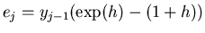 .
.
The local error is  because (from Taylor series)
 . The global error is
  : in fact,
on the
O and Order page, we used the example
: in fact,
on the
O and Order page, we used the example
 , which we saw had error . The
Euler approximation is just
, which we saw had error . The
Euler approximation is just  , so it too has error .
Another special case: suppose  is just a function of .
The true solution is
is just a function of .
The true solution is
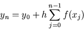
For the Euler method we have
 , so that
This is a just a Riemann sum for the integral: for each interval
![$[x_j, x_{j+1}]$](img64.png) we are approximating the area under the graph of
by a rectangle with height
we are approximating the area under the graph of
by a rectangle with height  . As you may have seen in
calculus, the error in this approximation for each interval is
at most
. As you may have seen in
calculus, the error in this approximation for each interval is
at most  if
if  on the interval, and the global
error at
on the interval, and the global
error at  is then at most
 .
.
Robert
2002-01-28