Reflection Functions

Ambient Reflection:

Ambient reflection is the simplest illumination model. There is no physical basic to the ambient term. It is the incoming light component that is identical everywhere in a scene. Ia is the global ambient illumination in the scene. Ka is the ambient reflection coefficient which is the amount of ambient light reflected from a surface. This model is a replacement for the true global illumination (light bouncing off from other objects).

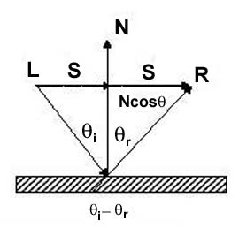
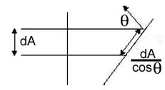
Ideal Specular: Mirror

It is the law of reflection. The reflection vector is calculated from mirroring L about N.

Both L and N are normalized. The projection of L onto N is Ncosθ. Through vector subtraction and congruent triangles S = Ncosθ - L. Thus, R = 2Ncosθ - L. Now, substitute N.L for cosθ: R = 2N.(N.L) - L.

Ideal Diffuse Reflection:

Diffuse or Lambertian reflection is exhibited by dull surfaces such as chalk. It is reflected light with an equal intensity in all directions. The brightness of a given surface depends only on the angle between the surface normal and the light source.

There are two effects to consider for the ideal diffuse reflection. First, the amount of light reaching the surface, this is dependent on cosθ . Second, the amount of light seen by the viewer, this is dependent of cosθ per unit surface area. The diffuse reflection is independent of viewing direction.

The diffuse lighting equation is:

If N and L are normalized:

The diffuse coefficient Kd is defined for each surface.

Specular Reflection:

Specular reflection can be observed on a shiny surface. Highlights as the colour of the light are observed on the surface of the object. The highlights appear in the direction of ideal reflection. Unlike diffuse, the view direction is important. Using the ideal mirror reflection from above, and adding n as the specular exponent the specular reflection equation is (known as the Blinn-Phong Model):

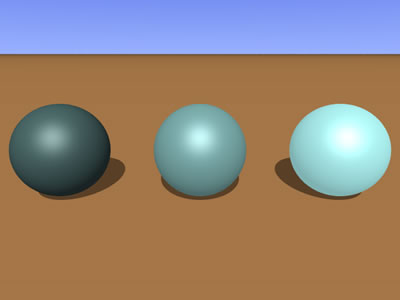
Some Examples

Below are some examples of the above models in use; alone and in combination.

From left to right, ambient values of 0.0, 0.5 and 1.0 in a 0 to 1 scale. Diffuse and Specular values are constant (diffuse 0.0, specular 0.0)

From left to right, diffuse values of 0.0, 0.5 and 1.0 in a 0 to 1 scale. Ambient and Specular values are constant (ambient 0.4, specular 0.0)

From left to right, specular values of 0.0, 0.5 and 1.0 in a 0 to 1 scale. Ambient and Diffuse values are constant (ambient 0.4, diffuse 0.0)

From left to right, ambient values of 0.2, 0.6 and 1.0 in a 0 to 1 scale. The specular and diffuse values constant at 0.4.

From left to right, diffuse values of 0.2, 0.6 and 1.0 in a 0 to 1 scale. The specular and ambient values constant at 0.4.

From left to right, specular values of 0.2, 0.6 and 1.0 in a 0 to 1 scale. The ambient and diffuse values constant at 0.4.